DIJKSTRA’S ALGORITHM

DIJKSTRA’S ALGORITHM

INTRODUCTION

In this short article I am going to show why Dijkstra’s algorithm is important and how to implement it. If you need some background information on graphs and data structure I would recommend reading more about it in Geeks for Geeks before reading this article. In any case I will try to be as clear as possible.

Before we get into this tutorial I would like to show you what the final result of our Dijkstra’s application will be:

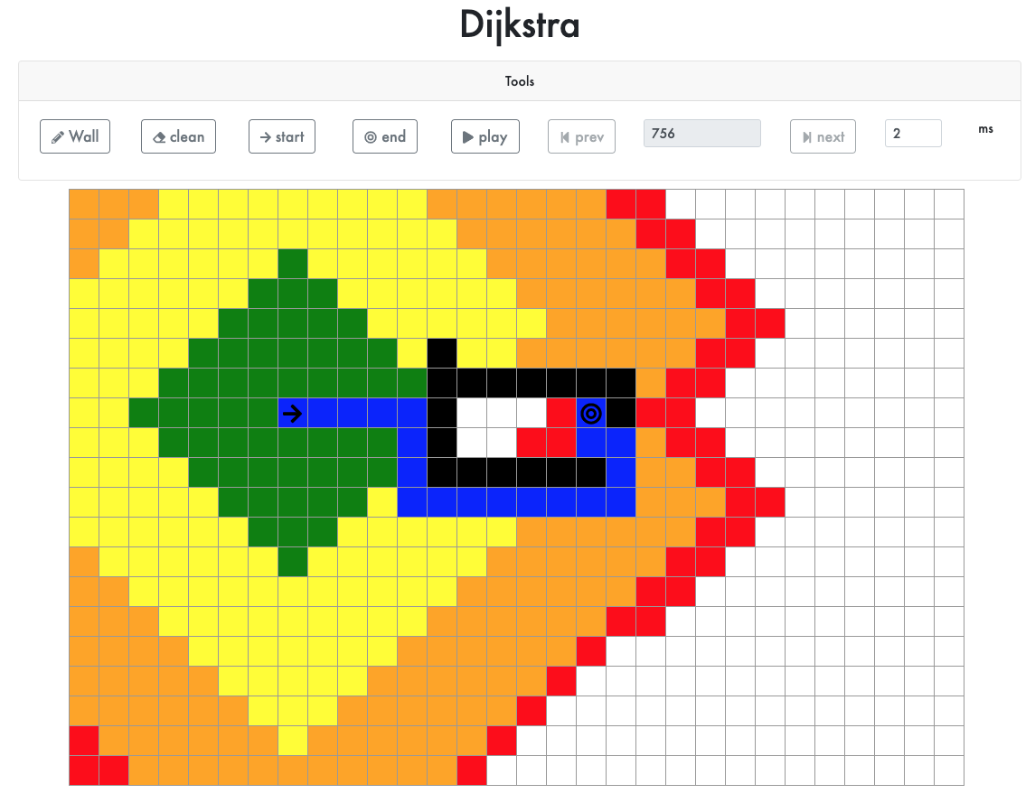
I decided to create a React application as I think that one of the best ways to learn a new concept is by seeing it in action.

WHY DIJKSTRA?

There are two reasons behind using Dijkstra’s algorithm. On one hand, it is a simple algorithm to implement. On the other hand one of the main features of this algorithm is that we only have to execute it once to calculate all the distances from one node in our graph and save it. This is a really important concept for future iterations where we will need to know what the shortest path from our init node is and we do not need to calculate it again, we can just use the previous calculated information, giving a really good performance.

For example, in the real world, we can use Dijkstra’s algorithm to calculate the distance between London and all the cities in the UK. Once this information is calculated and saved, we only have to read the previously calculated information. For example, looking at our data we can see what the shortest path from Norwich to London is. Later on in this article I will show you a real life example and how we can use previously calculated distances.

HOW IT WORKS

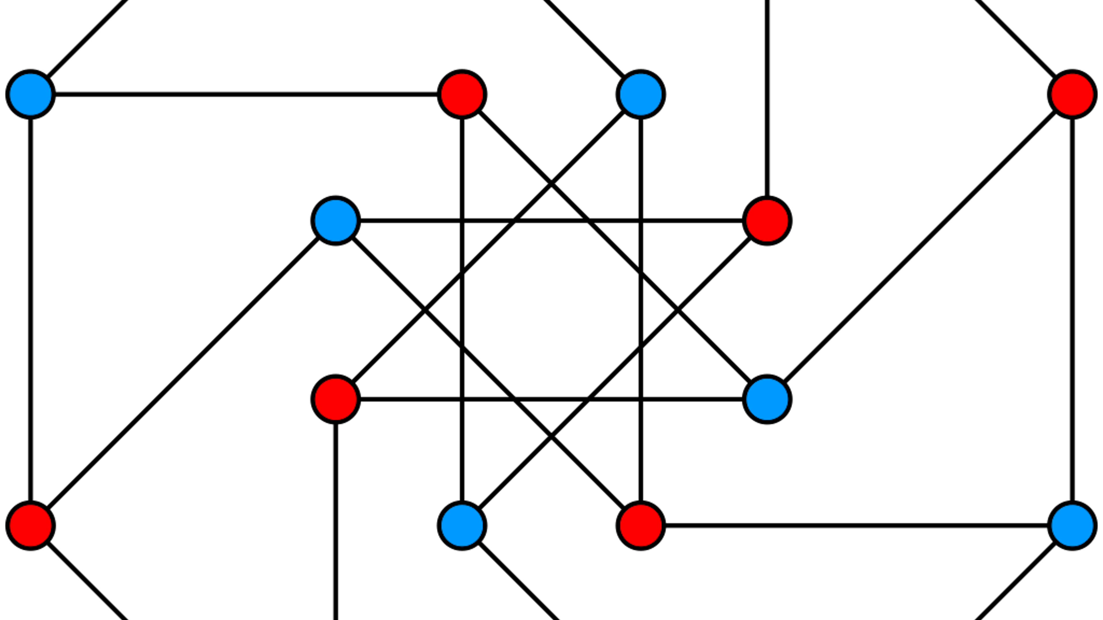
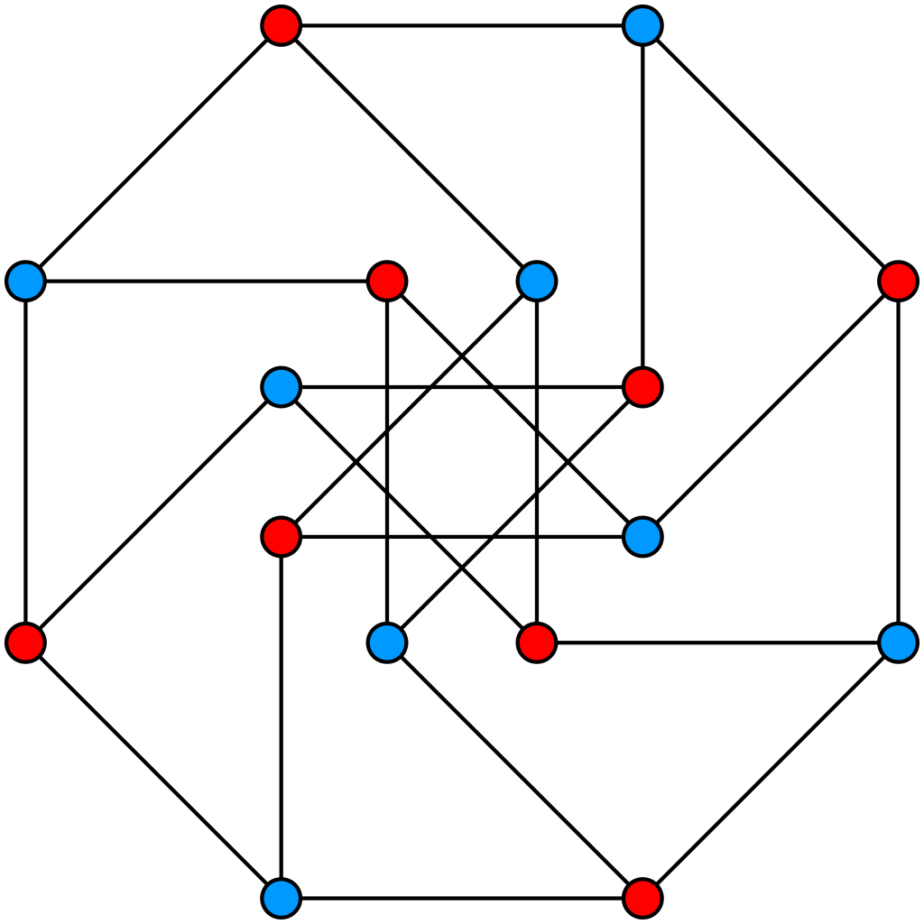
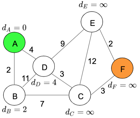
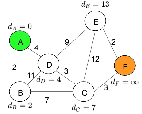
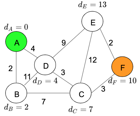
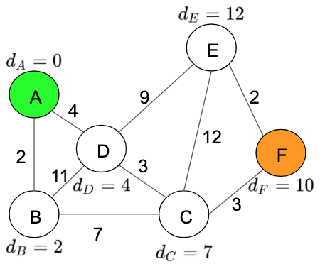
To explain how this algorithm works first I need to show you the graph that we are going to use in the rest of this section:

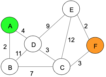
In the previous graph we can see 6 nodes from A-F, node A (highlighted green) is our start point and node F (highlighted orange) is our destination. Let’s now analyse this algorithm step by step:

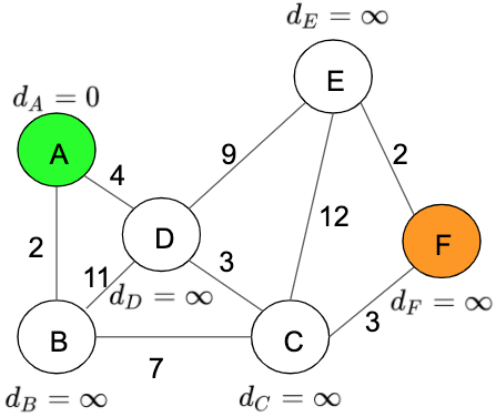
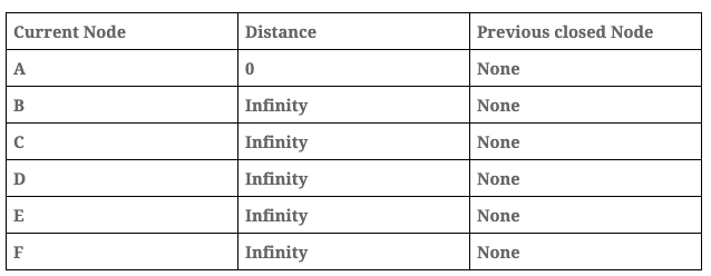
1. Initialise all the distances with the value infinite, except the initial node which is going to be initialized with the value 0.

Distance table:

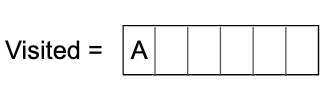
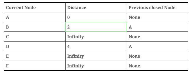
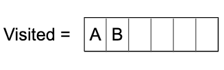
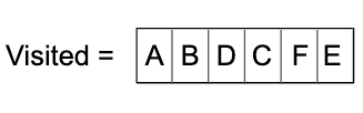
2. Add the current node, in this case ‘Node A’, into the visited array. We have to maintain this information to prevent analysing the same node more than once.

3. Calculate the distance between the current node and its children, the formula to calculate this distance is: total_distance = current_node_distance + path_distance, for example, between A and B the total_distant = 0 + 2 = 2. After this iteration the graph looks like this:

Distance table:

4. Now, analyse the next node. This node will be the no visited node with the minimum distance, in our case this node will be ‘Node B’. In this step we are going to repeat steps 2 and 3:

Distance table:

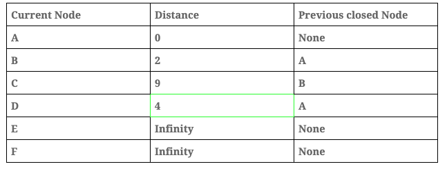
Important: the distance is updated only if the new distance is lower than the previous one. In this step the distance from B to D is 2 + 11 > 9, in this case the value remains at 9 because it is lower than 13.

5. After that, analyse the next node, the next node will be the no visited node with the minimum distance, in our case this node will be ‘Node D’. In this step we are going to repeat steps 2 and 3 again.

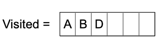
Distance table:

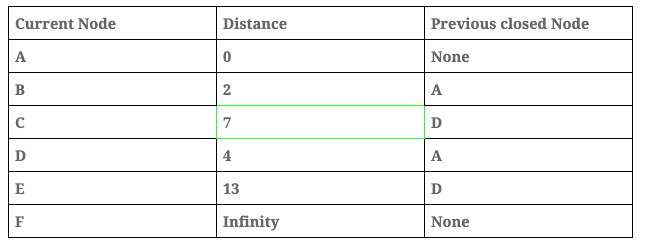
Important: the distance is updated only if the new distance is lower than the previous one. In this step the distance from D to C is 4 + 3 < 9, in this case the value changes to 7 and the previous node is now D.

6. We repeat the process this time with ‘Node C’.

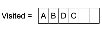
Distance table:

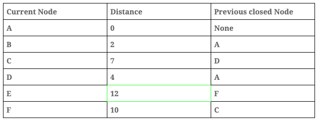
7. We repeat the process this time with ‘Node F’.

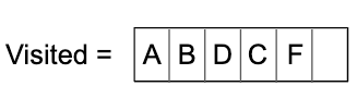
Distance table:

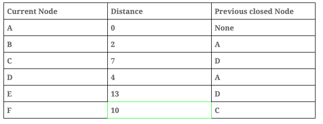
8. Finally, we analyse the last node in this case, ‘Node E’.

Distance table:

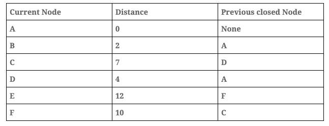
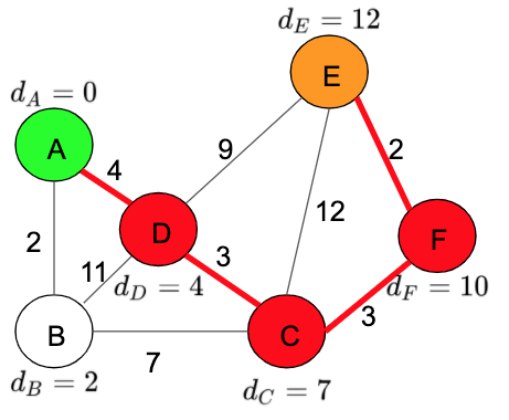
Now that we have our table with all the distances from ‘Node A’, we can find the shortest path from F. To do this, we have to find the distance from the current node F to Node A which is 10, and the path is calculated using the previous closed nodes results which are:

A -> D -> C -> F

As I said before, we can use the information in our table to find the shortest paths between A and any of the nodes in our graph. For example, between Node E and Node A the shortest path will be:

A -> D -> C -> F -> E

CODE IMPLEMENTATION

Data Structures

We are going to implement the previous algorithm using Typescript, as we have seen we need 2 main data structures to save the status:

export class Dijkstra {

    visited: Set<string>;
    dijkstraModelArray: Array<DijkstraModel>;
}

A Set, where we are going to save the visited node:

visited: Set<string>;

and an Array, where we are going to save the distances table data. In order to save this information we have created the following object:

export class DijkstraModel {

    private _currentNode: TreeNode;
    private _previousTreeNode: TreeNode | null;
    private _distant: number;
}

Algorithm

The implementation in our code is really similar to the steps I have shown you before. The only difference between our code and the steps explained is that in our code we stop as soon as we find the final node. The reason behind this decision is because we are not saving the information for future searches in order to simplify our code because the goal of this application is to show the algorithm, not the performance.

calculateShorterPath = (treeNodeArray: Array<TreeNode>) => {

        let currentNode: TreeNode | null = treeNodeArray[0];


        do {
            this.visited.add(currentNode.id);
            const distant: number = currentNode.distant;
            const currentDijkstra: DijkstraModel = new ...;
            this.dijkstraModelArray.push(currentDijkstra);
            this.iterateChild(currentDijkstra);
            currentNode = this.getNextNotVisitedNode();
        } while (!isNil(currentNode) && !currentNode.isEnd);

        if (isNil(currentNode)) return new DijkstraResModel([], []);

        const path: Array<Point> = this.createPath(currentNode);

        return new DijkstraResModel(this.dijkstraModelArray, path);
    }

We can see in our code the following steps:

1. Save visited node

2. Iterate child to calculate the distance

3. Find next minimum node not visited yet

4. Repeat until the end Node is found

5. Create path with the previously calculated information

CONCLUSION

In conclusion, Dijkstra’s algorithm is a really good starting point because it is simple yet efficient. This algorithm could be used in a variety of different situations such as IP routing, phone network routing, geographic maps and so on…

This implementation could be improved using concurrent, we can analyse the child nodes in parallels therefore improving performance. By following the enclosed video we can see a comparison between Dijkstra, A* and the concurrent Dijkstra algorithm.

REFERENCES

• Github code

• Graph data structure and algorithm

• Dijkstra wikipedia

• Dijkstra complexity time

• Introduction to algorithms

• Dijkstra’s Algorithm vs. A* Search vs Concurrent Dijkstra’s Algorithm